Crowdsensing the Census - Exploring Street Network
Last week we wanted to extract more information from Milan´s OSM data, so we performed visualization and analysis of its street network. We aim to find a relationship between the street connectivity and social deprivation. We also wanted to further investigate how this relationship differs from that of Milan in a city belonging to a developing country, particularly Mexico City.
One way to quantify the network of streets in a city, in terms of its connectivity is a network, or graph, with intersections as nodes and streets as edges connecting between the nodes
In order to compute connectedness of the street network, we calculated the two following graph centrality measures:
-
Betweenness centrality measures the number of shortest paths (streets, or edges) between any given pair of nodes (intersections) that pass through an individual node.
-
Closeness centrality measures how “close” you are to the center of the graph- that is, the length of average shortest path between a node and all nodes to the graph. For each node, the algorithm computes the length of the average shortest path between it and all the other nodes in the graph and calculates the inverse total length.
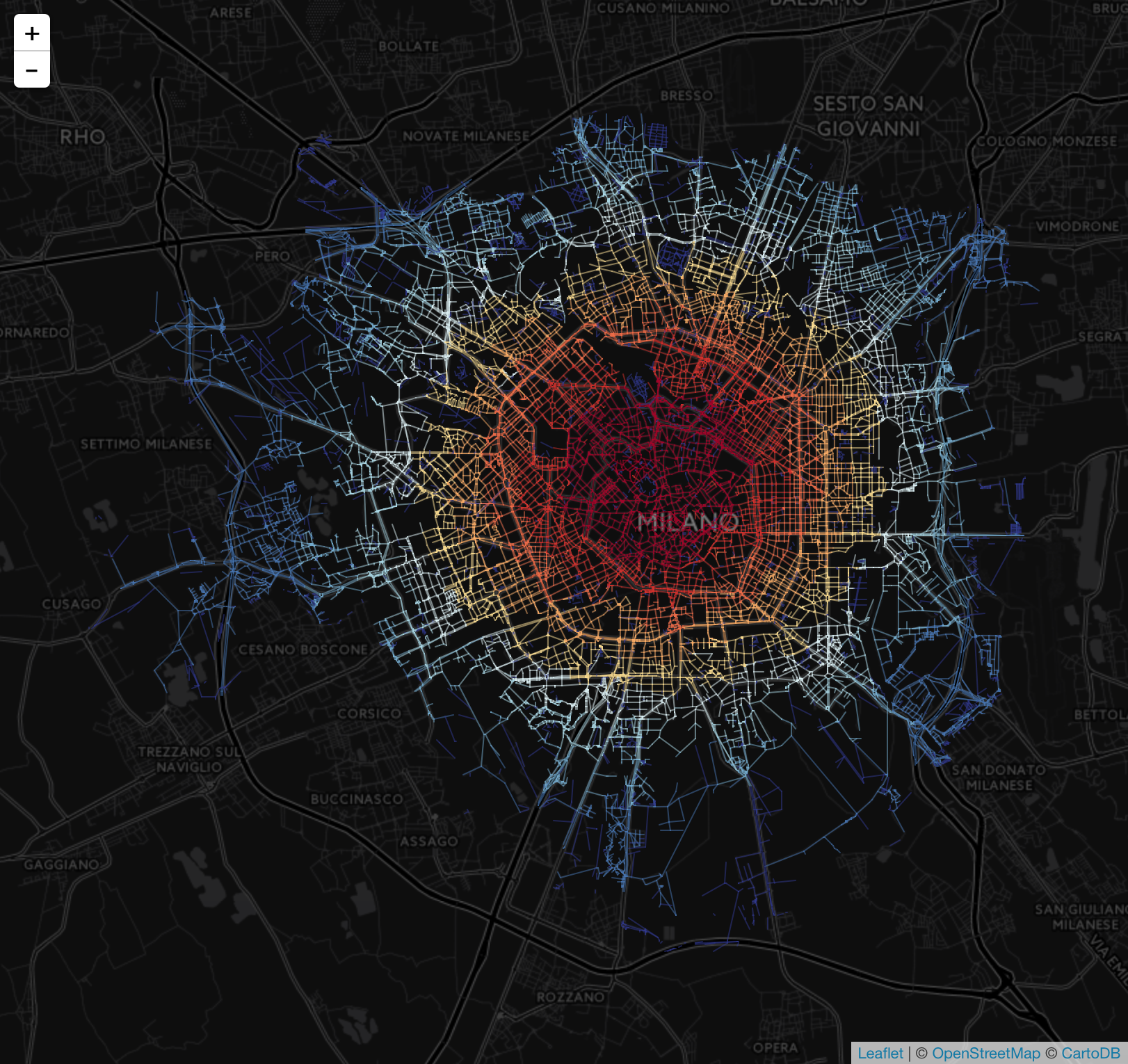
The following map shows both centrality measures for the city of Milan
| Closeness | Betweenness |
|---|---|
 |
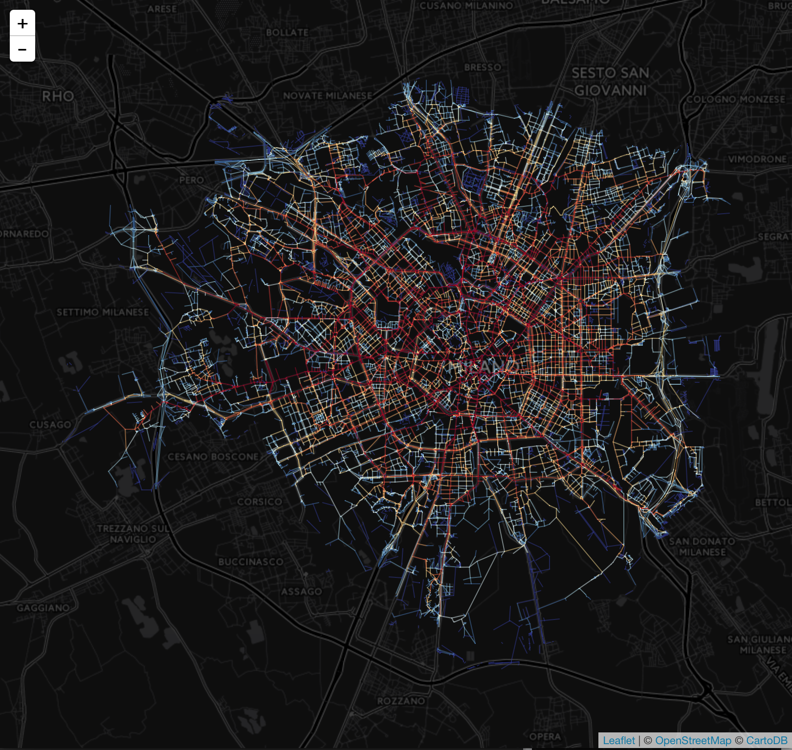 |
Each measure produces a different interpretation of the map. Closeness centrality exposes the radial structure of the streets where the highest centrality corresponds to the city center. Betweenness centrality provides a hierarchical view of the city where the main roads are highlighted in red (high centrality), and the streets between them are white/blue (low centrality).
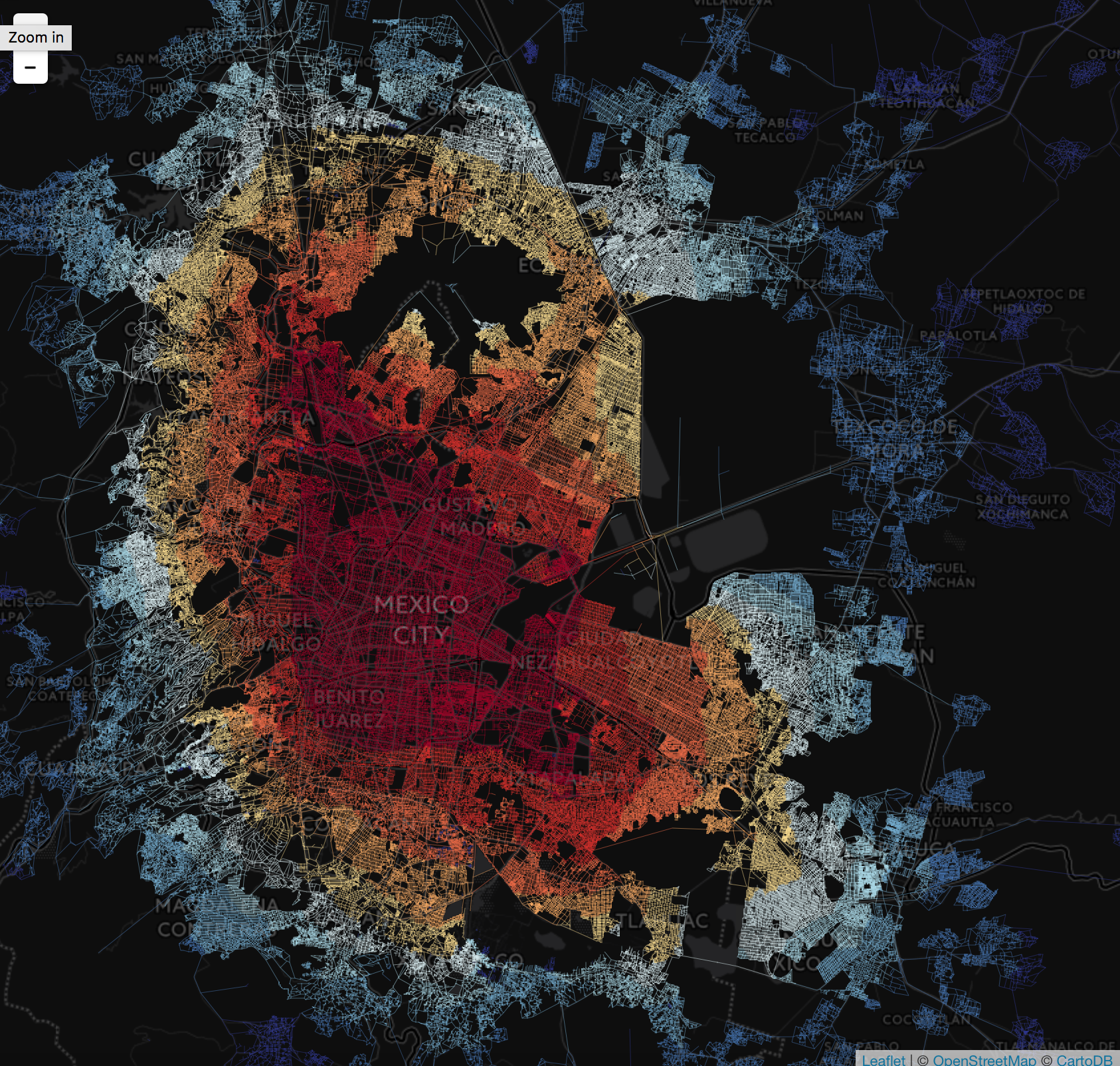
The following map shows both centrality measures for the city of Mexico City
| Closeness | Betweenness |
|---|---|
 |
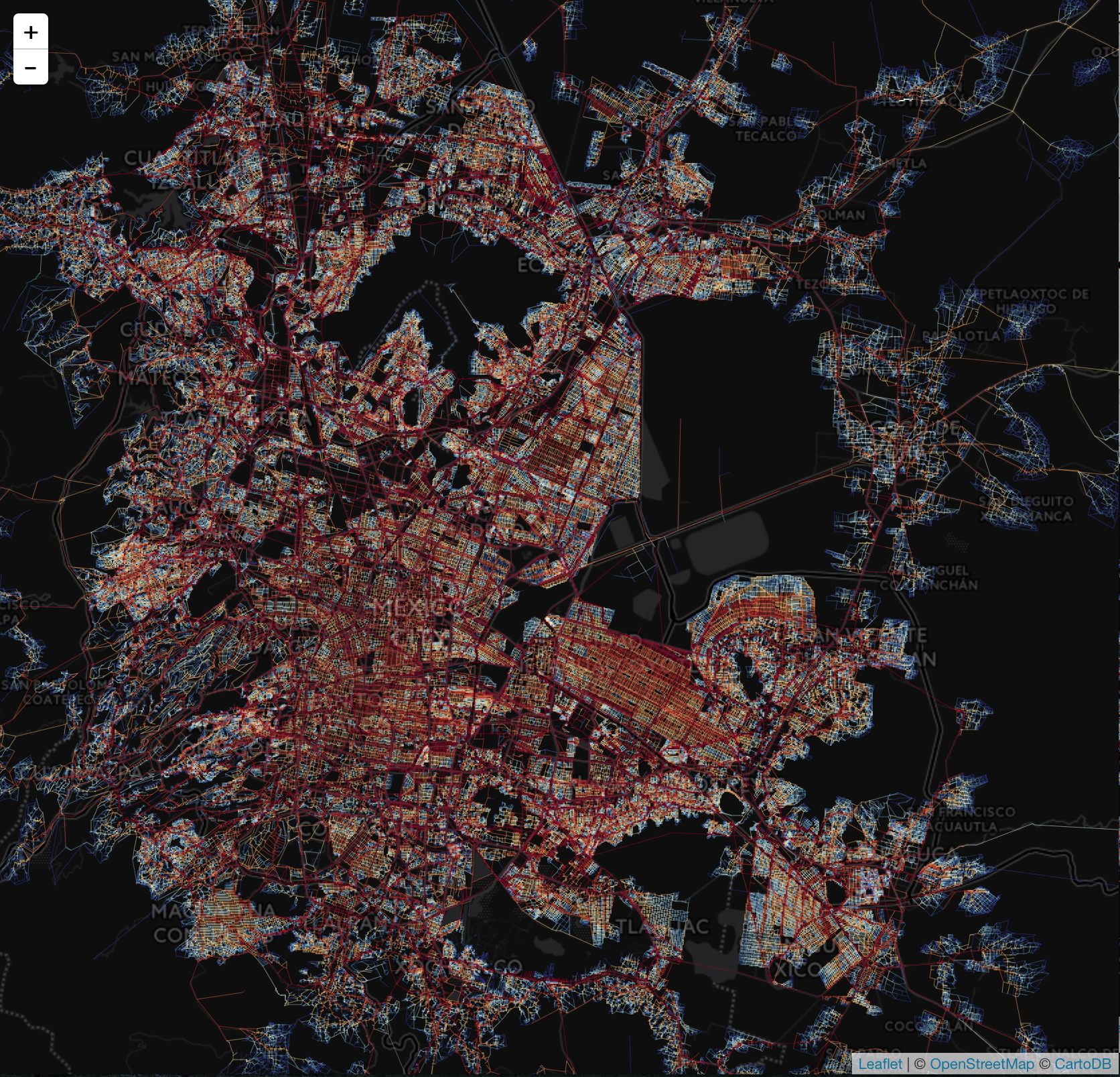 |
Mexico City does not have a radial structure, but closeness centrality highlights neighborhoods that are central to Mexico City in terms of economic significance, such as the Historic center and other established, affluent neighborhoods. Similar to Milan, betweenness centrality highlights main roads.
For the purpose of our project, we continued to analyze the relationship of the centrality measures in conjunction with deprivation. To achieve this, for each measure, we interpolated the nodes to a raster using inverse distance weighting (IDW) and then aggregated the raster to each census polygon using the median. It is also possible to aggregate using other measures like mean, max, range, etc.
First, we explored the relationship between the street network centrality and our Milan well-being index:
| correlation | p-value | |
|---|---|---|
| closeness | 0.094 | 0.39 |
| betweenness | 0.069 | 0.53 |
Table: Correlation between centrality measures and well-being index in Milan The correlations are clearly not significant in the case of Milan. In the case of Mexico City, however:
| correlation | p-value | |
|---|---|---|
| closeness | -0.49 | <2e-16 |
| betweenness | -0.39 | <2e-16 |
Table: Correlation between centrality measures and deprivation index in Mexico City
Both measures exhibit a significant inverse correlation with the deprivation index. This means that the areas with more street network centrality, on average, are less deprived.
From our results, we can see that in Mexico City the connectivity is related to deprivation. This may be because Mexico City is a sprawling metropolis that is spread out across a large area. This makes commutes for people in less central areas extremely long, and therefore the more central residential areas are most desirable in terms of convenience. Housing costs are highest in the central region, thus resulting in higher levels of deprivation in the outskirts and more suburban areas.