Preliminary Classification
For the initial classification model, we implemented the review text as the model features- that is, the model accounted for common terms to determine whether a review should be tagged as linked to a recalled product or not. We began with 4 different models to test. We tested both L1 and L2 logistic regression models. L1 and L2 regularization are different ways to handle irrelevant features, or noise. L1 works better usually when there are many, many features, because it handles an exponential growth in irrelevant features, which is likely what our data would exhibit. We also tested a Linear Support Vector Machine classification model and a Ridge Regression model. Since models with a lot of features, such as term frequencies, tend to be linearly separable, these two linear models were potentially good fits for our data. Both regularize the weights to avoid over-fitting.
Supervised Learning Evaluation
Below are the results from our initial testing of the 4 models. All text in the reviews are evaluated as model features, and each definition of recall (review +/- 6 months from recall date, review +/- 1 year from recall date, review 1 year before recall date, review 6 months before recall date) is evaluated as the dependent variable. Model accuracy, precision, recall, and F1-score is evaluated for each model/dependent variable combination using a 50% test/train split.
Review +/- 1 Year from recall:
| Accuracy Measure | Regression- L1 | Regression- L2 | Linear SVC | RidgeRegression |
|---|---|---|---|---|
| Accuracy | 0.849 | 0.853 | 0.818 | 0.840 |
| Precision | 0.614 | 0.630 | 0.473 | 0.563 |
| Recall | 0.343 | 0.371 | 0.442 | 0.353 |
| F1 | 0.440 | 0.467 | 0.457 | 0.434 |
Review 6 months before recall:
| Accuracy Measure | Regression- L1 | Regression- L2 | Linear SVC | Ridge Regression |
|---|---|---|---|---|
| Accuracy | 0.947 | 0.948 | 0.923 | 0.942 |
| Precision | 0.174 | 0.233 | 0.120 | 0.102 |
| Recall | 0.045 | 0.056 | 0.107 | 0.034 |
| F1 | 0.072 | 0.091 | 0.113 | 0.051 |
Review +/- 6 Months from recall:
| Accuracy Measure | Regression- L1 | Regression- L2 | Linear SVC | Ridge Regression |
|---|---|---|---|---|
| Accuracy | 0.920 | 0.920 | 0.896 | 0.919 |
| Precision | 0.384 | 0.378 | 0.258 | 0.364 |
| Recall | 0.133 | 0.129 | 0.220 | 0.126 |
| F1 | 0.197 | 0.193 | 0.238 | 0.187 |
Review 1 year before recall:
| Accuracy Measure | Regression- L1 | Regression- L2 | Linear SVC | Ridge Regression |
|---|---|---|---|---|
| Accuracy | 0.887 | 0.888 | 0.860 | 0.881 |
| Precision | 0.438 | 0.451 | 0.334 | 0.380 |
| Recall | 0.203 | 0.210 | 0.319 | 0.184 |
| F1 | 0.277 | 0.287 | 0.326 | 0.248 |
We mostly care about the recall measure (the % of recalled product reviews identified), given that our data are imbalanced. Therefore, Linear SVM with the review being +/- 1 year from the recall performed the best. However, there is definitely still needed improvement to our model.
Key Words and Performance of Linear SVM
The next task was to investigate key words (features) in the model that held the most weight. In this exercise, we performed 20-fold cross-validation to give more credibility to our model, while also extracting the top 10 most predictive words. We also separated our training and test set to not include reviews for the same product in both data subsets. This way, we could account for product-specific noise.
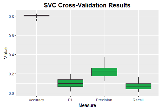
| Measure | Min. | 1st Qu. | Median | Mean | 3rd Qu. | Max. |
|---|---|---|---|---|---|---|
| Accuracy | 0.754 | 0.799 | 0.807 | 0.8028 | 0.8145 | 0.825 |
| Precision | 0.126 | 0.1762 | 0.228 | 0.2275 | 0.2638 | 0.375 |
| Recall | 0.008 | 0.0405 | 0.0625 | 0.07615 | 0.1 | 0.165 |
| F1 | 0.015 | 0.06575 | 0.0995 | 0.1055 | 0.1418 | 0.198 |
Most Predictive Terms
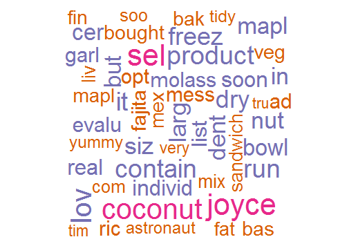
We are getting some low recall values, and it looks like product-specific terms (e.g., coconut) are getting a lot of weight in the models. This means that our model may have a hard time being generalizable - lets look at the full model (i.e., no cross validation) to see the terms that are getting the most weight when using all products
| Term | Coef | |
|---|---|---|
| 3804 | gingerbread | 1.697815 |
| 4921 | justins | 1.639414 |
| 6709 | paprik | 1.629455 |
| 7407 | quinoa | 1.571956 |
| 3951 | granddaught | 1.525153 |
| 3241 | fajita | 1.496793 |
| 288 | amino | 1.482580 |
| 7504 | recal | 1.444783 |
| 10264 | wash | 1.374378 |
| 4066 | guav | 1.362638 |
| 8381 | skippy | 1.324039 |
| 701 | basil | 1.316200 |
| 7406 | quino | 1.306519 |
| 8095 | seam | 1.296897 |
| 1955 | concoct | 1.280640 |
| 6217 | newton | 1.277910 |
| 4264 | hent | 1.277887 |
| 6332 | nugo | 1.252936 |
| 7437 | ram | 1.234634 |
| 10201 | vs | 1.229726 |
| 3543 | foul | 1.216128 |
| 8410 | slightly | 1.190934 |
| 5288 | lightn | 1.181437 |
| 32 | accid | 1.172457 |
| 7016 | plum | 1.166517 |
| 2945 | eldest | 1.129980 |
| 6433 | oi | 1.122017 |
| 4009 | greek | 1.108895 |
| 1170 | broth | 1.106454 |
| 10050 | variety | 1.090841 |
| 9354 | terrible | 1.082349 |
| 6303 | note | 1.080769 |
| 9199 | taco | 1.077790 |
| 7780 | rins | 1.077001 |
| 2697 | doct | 1.069091 |
| 5261 | lic | 1.059215 |
| 509 | assum | 1.049675 |
| 8014 | sazon | 1.044622 |
| 2868 | easiest | 1.030123 |
| 917 | blackstrap | 1.027565 |
| 1931 | completely | 1.026621 |
| 9512 | tid | 1.019473 |
| 281 | america | 1.016342 |
| 1817 | co | 1.013590 |
| 10569 | yay | 1.008432 |
| 4197 | hazelnut | 1.007850 |
| 2305 | daddy | 1.004679 |
| 801 | belvita | 1.001835 |
| 2033 | conv | 1.000000 |
| 10662 | zicos | 1.000000 |
Terms in the model are (mostly) product specific - so let’s take a look at how precision (ability of the model to NOT label non-recalled products as a recalled product) and information recall (ability of the model to detect all recalled product reviews) interact. Again, cross validation is used where sets include different product IDs.
##Precision Recall Curve
from sklearn.metrics import precision_recall_curve, average_precision_score
import seaborn as sns
from sklearn.cross_validation import LabelKFold
import matplotlib.pyplot as plt
%matplotlib inline

labels = np.array(Subset.asin)
lkf = LabelKFold(labels, n_folds=10)
lr = LogisticRegression(C=C, penalty='l2')

plt.figure(figsize=(10,7))

for i, (train, test) in enumerate(lkf):
    y_score = lr.fit(text_matrix[train], \
                target[train]).decision_function(text_matrix[test])
    precision, recall, _ = precision_recall_curve(target[test], y_score)
    average_precision = average_precision_score(target[test], y_score)
    plt.plot(precision, recall, lw=1, label='Curve for fold %d (area = %0.2f)' \
             % (i+1, average_precision))

sns.set(style="darkgrid", color_codes=True, font_scale=1.25, palette='bright')
plt.xlim([0.0, 1.0])
plt.ylim([0.0, 1.0])
plt.xlabel('Recall')
plt.ylabel('Precision')
plt.title('Precision Recall Curve - Logistic Regression with 10 CVs')
plt.legend(bbox_to_anchor=(1.05, 1), loc=2, borderaxespad=0.)
plt.show()
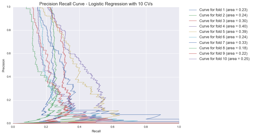
We see that precision is driven to zero with only a slight increase in information recall. This means that in order to identify even 20% of recalled products across product-types, we must label almost all non-recalled products as being recalled (which is not what we want!)
Evaluate Model with Generic Terms
Among all terms that were predictive of a recalled product review, there was a subset of terms that were in line with foodborne-illness symptoms and food-spoilage. These terms were pulled out and the model was re-evaluated in order to see the performance with only these therms.
##Create Word List that only includes non-product specific terms

word_list = ['detect', 'deceiv', 'recal', 'unus', 'foul', 'gassy', 'vomit', 'tummy', 'horr', 'horrend', 'disbeliev', 'hesit', 'annoy', \
'lie', 'distress', 'projectil', 'intestin', 'bitter',  'complaint', 'bad', 'urin', 'ridic', 'gross', \
'frust', 'rot', 'runny', 'terrible', 'unfortun', 'waste', 'throw', 'sour', 'batch', 'misl', 'mislead', 'unsatisfy', 'puk', \
'watery', 'lousy', 'wrong', 'undrinkable', 'stinky', 'bacter', 'wtf', 'celiac', 'parasit', 'discomfort' \
'nausea', 'naus', 'nause', 'pung', 'label', 'ingest', 'sick', 'throwing', 'dislik', 'defect', 'indescrib',\
'screwed', 'fridg', 'diogns', 'decad', 'flourless', 'dissatisfy', 'infect', 'disgruntl', 'disgusting', 'disgust',\
'rancid', 'cramp', 'nasty', 'underflav', 'allerg', 'nondairy', 'burnt', 'toss', 'yuck', 'awful', 'funny', 'victim', \
'queasy', 'mush', 'dissapoint', 'alarmingly', 'gluten', 'esophag', 'cloudy', 'unsuspect']

vectorizer_subset = CountVectorizer(binary=False, ngram_range=(1, 1), vocabulary=word_list)
text_matrix2 = vectorizer_subset.fit_transform(final_text)
##Plot summation of features vs. classification
import scipy
from scipy.sparse import coo_matrix
import seaborn as sns
import matplotlib.pyplot as plt
%matplotlib inline

vectorizer_excludeRecallkeywords = CountVectorizer(binary=False, ngram_range=(1, 1), stop_words=word_list)
food_review_text_sum = vectorizer_excludeRecallkeywords.fit_transform(final_text)
food_review_text_sum = scipy.sparse.coo_matrix.sum(food_review_text_sum, axis=1)
counts_recallwords = scipy.sparse.coo_matrix.sum(text_matrix2, axis=1)
df_for_graph = pd.concat([pd.DataFrame(counts_recallwords, columns=['recallWords']), \
                          pd.DataFrame(food_review_text_sum, columns=['otherWords']),\
                          pd.DataFrame(target, columns=['target'])], axis=1)


sns.set(style="darkgrid", color_codes=True, font_scale=1.25, palette='bright')
plt.xlim(-0.1,15)
plt.ylim(-0.1, 600)
plt.title('Recall Keywords vs. All Other Words')
plt.xlabel('Sum of Recall Keyword Frequency')
plt.ylabel('Sum of All Other Words Frequency')
plt.scatter(df_for_graph[df_for_graph.target==1].recallWords, df_for_graph[df_for_graph.target==1].otherWords,\
            marker='o', c='g', label='Recalled')
plt.scatter(df_for_graph[df_for_graph.target==0].recallWords, df_for_graph[df_for_graph.target==0].otherWords,\
            marker='o', c='b', label='Not Recalled')
plt.tight_layout()
plt.legend(bbox_to_anchor=(1, 1), loc=2)

##Test model using cross validation
from sklearn import cross_validation
target = np.array(Subset.recalled_1y)

scores = cross_validation.cross_val_score(model, text_matrix2, target, cv=50)
print("Mean Model Accuracy with 50 CV: %0.5f (+/- %0.5f)" % (scores.mean(), scores.std() * 2))

text_matrix2test, text_matrix2train, Y_test, Y_train = train_test_split(text_matrix2, target, test_size=0.5, random_state=123)
model.fit(text_matrix2train, Y_train)
Y_pred = model.predict(text_matrix2test)
print("Precision: %1.3f" % precision_score(Y_test, Y_pred))
print("Recall: %1.3f" % recall_score(Y_test, Y_pred))
print("F1: %1.3f\n" % f1_score(Y_test, Y_pred))
Mean Model Accuracy with 50 CV: 0.83270 (+/- 0.01640)
Precision: 0.378
Recall: 0.025
F1: 0.047
from sklearn.metrics import roc_curve, auc
from scipy import interp
sns.set(style="darkgrid", color_codes=True, font_scale=1.25, palette='bright')
# Run classifier with cross-validation and plot ROC curves
mean_tpr = 0.0
mean_fpr = np.linspace(0, 1, 100)
all_tpr = []
for i, (train, test) in enumerate(lkf):
probas_ = lr.fit(text_matrix2[train], target[train]).predict_proba(text_matrix2[test])
# Compute ROC curve and area the curve
fpr, tpr, thresholds = roc_curve(target[test], probas_[:, 1])
mean_tpr += interp(mean_fpr, fpr, tpr)
mean_tpr[0] = 0.0
roc_auc = auc(fpr, tpr)
plt.plot(fpr, tpr, lw=1, label='ROC fold %d (area = %0.2f)' % (i+1, roc_auc))
plt.plot([0, 1], [0, 1], '--', color=(0.6, 0.6, 0.6), label='Luck')
mean_tpr /= len(lkf)
mean_tpr[-1] = 1.0
mean_auc = auc(mean_fpr, mean_tpr)
plt.plot(mean_fpr, mean_tpr, 'k--',
label='Mean ROC (area = %0.2f)' % mean_auc, lw=2)
plt.xlim([0.0, 1.05])
plt.ylim([0.0, 1.05])
plt.xlabel('False Positive Rate')
plt.ylabel('True Positive Rate')
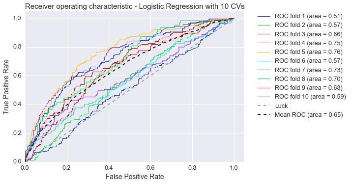
plt.title('Receiver operating characteristic - Logistic Regression with 10 CVs')
plt.legend(bbox_to_anchor=(1.05, 1), loc=2, borderaxespad=0.)
plt.show()

The ROC curve demonstrates that the model with generic terms is only approximately 50% accurate when evaluating across products. This is partially due to the problem that the reviews are very short and none of the words we have selected are contained in the text. This urged us to test the classification with all words as features which increased the average performance to 65%, as it can be seen in the plot below.
Non-linear Model
In our initial classification experiments, we also attempted to see the success of a non-linear model. In this case, we selected the Random Forest Classifier.
##Random Forest
from sklearn.ensemble import RandomForestClassifier
target = np.array(Subset.recalled_1y)

rfc = RandomForestClassifier(n_estimators=200, criterion='entropy')
nonlinear_results = rfc.fit(text_matrix, target)
##Find Important Terms
importance = np.transpose(nonlinear_results.feature_importances_)
importance_df = pd.DataFrame(importance, columns=['Importance'])
importance_df = pd.concat([term_names, importance_df], axis = 1)
importance_df = importance_df.sort_values(by='Importance', ascending=False)
importance_df[importance_df.Importance > 0].head(n=20)
| Term | Importance | |
|---|---|---|
| 1832 | coconut | 0.017936 |
| 7406 | quino | 0.011562 |
| 9297 | tea | 0.009681 |
| 1840 | coff | 0.008188 |
| 7111 | pouch | 0.006762 |
| 10269 | wat | 0.005521 |
| 5419 | lov | 0.005250 |
| 3895 | good | 0.005139 |
| 7407 | quinoa | 0.004978 |
| 9264 | tast | 0.004937 |
| 5294 | lik | 0.004822 |
| 7237 | produc | 0.004637 |
| 3419 | flav | 0.004578 |
| 10006 | us | 0.004496 |
| 3995 | gre | 0.004316 |
| 2874 | eat | 0.003891 |
| 6462 | on | 0.003863 |
| 6794 | peanut | 0.003759 |
| 9459 | this | 0.003620 |
| 1261 | but | 0.003578 |
##Statistics of the model
X_test, X_train, Y_test, Y_train = train_test_split(text_matrix, target, test_size=0.5, random_state=123)
rfc.fit(X_train, Y_train)
Y_pred = rfc.predict(X_test)
print("\tAccuracy: %1.3f" % accuracy_score(Y_test, Y_pred))
print("\tPrecision: %1.3f" % precision_score(Y_test, Y_pred))
print("\tRecall: %1.3f" % recall_score(Y_test, Y_pred))
print("\tF1: %1.3f\n" % f1_score(Y_test, Y_pred))
	Accuracy: 0.841
	Precision: 0.788
	Recall: 0.116
	F1: 0.202
As we can see, non-linear models also have the challenge of identifying product-specific terms and having a low proportion of recalls identified.
Future Directions
There is still wide margin for improvement, and we need custom designed algorithms to extract the right features. However, initial exploration of the text showed that there exist features that indicate necessity for recall. It is a matter of selecting the right features that add weight to the most important aspects of the text.
We have already performed exploratory analysis of other aspects of the data in hopes of implementing into a (hopefully) better classification model. We have researched ways to implement the product categories as a feature in order to account for all of the product-specific noise. Also, we have researched the corresponding FDA data and developed useful topics from the Reason for Recall text data. We have yet to determine if these are worthwhile features to include. Stay Tuned!
To see a full notebook with all of our code to date of the supervised model, click here.