Measuring streaks
When an image does contain a streak, its plotted median pixel intensity values will look approximately Gaussian.
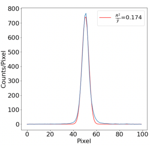 This plot shows the median pixel intensity values from an image with a streak. The blue line represents the real data from the image, which looks approximately Gaussian. We fit a line through the real data, which is represented by the red line.
We empirically determined appropriate fitting thresholds that perform well for all the image data we have available (we manually vetted this for at least a dozen images). When we fit a Gaussian profile to a real streak, we require the normalized root mean squared deviation, distance from the center of the cutout, and full width half maximum all pass the our thresholds. If the fit converges and passes validation, we confirm we have measured a streak.
When we have a good fit that passes validation, we keep this data and measure streak properties such as mean brightness scaled to the pixel level of the image, amplitude, which represents the median brightness of the streak, the full width half maximum, which represents the width of the streak, and the standard deviation (sigma) value of the fitted Gaussian.
Refining the rotation angle
Rotating images around the mean of the cluster of detected Hough lines, as we do for validation, finds only an approximate rotation angle for the line. As a result, the line in the rotated image is not necessarily perfectly horizontal. This negatively affects the precision of our measurements.
To improve this, we rotate the cutout image containing a streak around its calculated mean angle and repeat the fitting procedure to see which angle gives us the most accurate fit. We adopt the angle that returns the straightest line as the refined rotation angle.
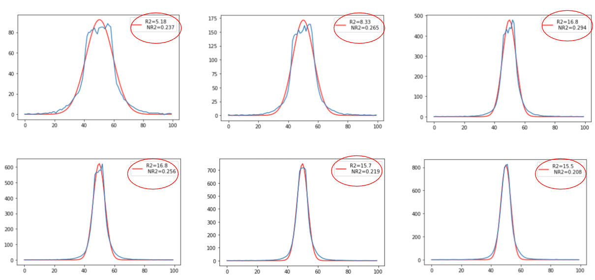 The plots above are 6 rotated iterations of one image. We fit a line through each iteration and empirically determined that an image with a smaller normalized root mean square deviation is more representative of a straighter streak. The bottom right image has the lowest normalized root mean squared deviation and its line is fitted very closely to the real data. As a result, we would accept the angle that the bottom right plot has for our rotation angle that straightens our line
We tested this technique by applying the Gaussian fitting function on each of the profiles generated from slightly different rotation angles. We assume an image with a smaller normalized root mean squared deviation is more representative of a straighter streak. This process has helped us refine the algorithm and measure our streak properties with more accuracy.
Edge cases
In certain cases, the line enters and/or exists in the image in such a position that it is impossible to effectively crop out the line without including the edge of the image in the cutout or excluding a section of the trail. For example, this can occur when a trail is close and parallel to the edge of an image.
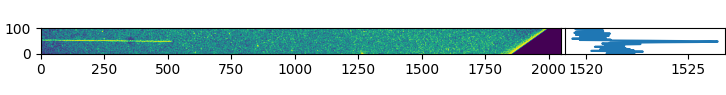 Image cutout containing the edge of the image. The profile on the right shows an obvious trend due to the edge
Excluding a section of the trail risks cutting the trail so short that it becomes undetectable and includes the image edge in the cutout, which biases our profile. To combat this, we remove any outliers from the retrieved profile by applying sigma clipping and fit a line to the remaining points. We then subtract the mean trend from our data, effectively removing the bias introduced by including the edge of the image in the cutout.
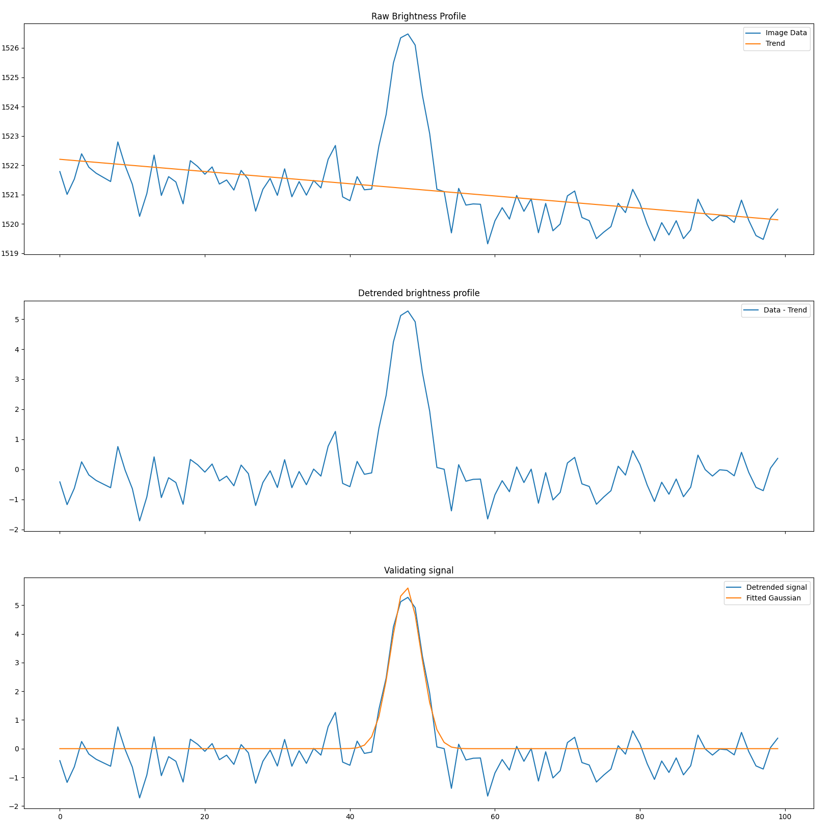 The same profile as in the above figure is shown in blue in the top plot. In orange in the top plot is our fitted trend line. The middle plot represents the detrended image profile, i.e the image profile minus the fitted trend. The last plot shows our fit for the Gaussian streak profile
After detrending and refining the rotation angle, Satmetrics outputs the fit parameters of the image alongside with statistics such as mean pixel intensity of the trail, filename and other information back to the user in YAML format.